Government Positions from Party-Level Data
Dimiter Toshkov (@DToshkov)
30 January, 2019
Introduction
In empirical research in political science and public policy we often need estimates of the ideological and policy positions of governments. However, the existing data sources typically provide data at the level of political parties. This document presents one way to derive government positions from party-level data using the Manifesto Project party-level data and combining it with data on the duration and composition of governments from the ParlGov database. The approach is implemented in the R language and environment for statistical computing and graphics.
Using the approach described below, you can easily derive government positions from Manifesto data based on existing scales, but you can also create your own scale by combining individual items from the Manifesto corpus. You can use different ways of scaling the items. And you can obtain the resulting estimates aggregated by cabinet, by year, and by month. All the necessary functions to do that are defined and described below, but they are not collected in a self-contained package yet.
These are the main steps in this tutorial:
- Load the original datasets
- Do some work to align the datasets before merging them
- Define functions to compute new party-level positions and scales
- Define functions to aggregate party positions into government positions
- Define functions to aggregate government positions into time series by month or by year
All functions and suppporing code presented in this text are deposited on GitHub. You are welcome to contribute by streamlining the code, idetifying and correcting mistakes or suggesting new features to add. Here is a link to the GitHub repository of the project.
Let’s get started: packages and functions
The first thing to do is load the packages that we gonna need. I like this way of installing and loading packages: first load (or install first if needed) the install.load package, and then use this package to load (or install first if needed) the remaining ones.
if (!require(install.load)) {
  install.packages("install.load", repos = "http://cran.us.r-project.org")
  require(install.load)
}

install_load("reshape2", "manifestoR", "readr", "countrycode", "zoo", "lubridate", "devtools")
Second, we gonna need to define some basic general functions. The first one is just a shorthand to transform factors and character vectors into actual numbers and to round the numbers if needed. The other functions customize the basic and by-row summation, averaging, minimum, and maximum functions by letting them ignore missing data (which is not their default behavior). Note that when the na.rm=T argument is included, summing (or other operations such as taking the mean or the minimum) over a vector of NAs will return a zero, not NA. This is not always what we want, so we better have versions of the functions that ignore individual NAs but return ‘NA’ if there are no valid observations to work with.
make.number<-function (x, y) {round(as.numeric(as.character(x)), digits=y)}

sum.na<-function (x) sum(x, na.rm=T) #sum that aviods NAs, returns 0 if all NAs
sum.allna <- function(x) if (all(is.na(x))) NA else sum(x,na.rm=T) #sum that avoids NAs but returns NA if all NAs

rowsum.na<-function (x) rowSums(x, na.rm=T) #sum by row that avoids NAs
rowsum.allna <- function(x) rowSums(x, na.rm=TRUE) * ifelse(rowSums(is.na(x)) == ncol(x), NA, 1) #sum by row that avoids NAs but gives NA for a row with all NAs

mean.na<-function (x) mean(x, na.rm=T) #sum that aviods NAs, returns infinity if all NAs
mean.allna <- function(x) if (all(is.na(x))) NA else mean(x,na.rm=T) #sum that avoids NAs but returns NA if all NAs

min.na<-function (x) min(x, na.rm=T) #sum that aviods NAs, returns 0 if all NAs
min.allna <- function(x) if (all(is.na(x))) NA else min(x,na.rm=T) #sum that avoids NAs but returns NA if all NAs

max.na<-function (x) max(x, na.rm=T) #sum that aviods NAs, returns 0 if all NAs
max.allna <- function(x) if (all(is.na(x))) NA else max(x,na.rm=T) #sum that avoids NAs but returns NA if all NAs

## we can also source the functions from a local file or from the GitHub repository of this project
#source('basic general functions.r')
#source('https://raw.githubusercontent.com/demetriodor/govpositions/master/basic%20general%20functions.R')
Getting the original datasets
We are ready to load the original datasets that we gonna use to derive the government positions. We gonna need the Manifesto Corpus data, which we can obtain via its R package, and the ParlGov data, which we can get directly from the web. We need two datasets from ParlGov: one for parties, which contains the codes to link to the Manifesto data, and one for cabinets, which provides the data on cabinet duration and composition. To access the Manifesto data, you will need to get your own API key by signing up to their webpage and then logging in to your account (see here for details).
mp_setapikey("manifesto_apikey.txt") #set up the API key for access to the Manifesto data
manifestos <- mp_maindataset() #loads the most current version by default, right now this is version 2018-2, '2018b'
## Connecting to Manifesto Project DB API...
## Connecting to Manifesto Project DB API... corpus version: 2018-2parties<-read_csv('http://www.parlgov.org/static/data/development-utf-8/view_party.csv') #ParlGov party-level file
cabs <-read_csv('http://www.parlgov.org/static/data/development-utf-8/view_cabinet.csv') #ParlGov cabinets-level fileWe can subset only the relevant columns and countries. My focus is on the European countries, so I list the ISO3 codes of the 28 member states of the EU plus Iceland, Norway, and Switzerland. The countrycode function translates the ISO3 country codes to country names. The Czech Republic officially changed its name to ‘Czechia’, so we better change it in the datasets as well.
#subset only relevant columns
parties<-parties%>%select(country_name, party_name_english,party_id, cmp)
cabs<-cabs%>%select      (country_name, party_name_english, party_id,
                          cabinet_id, previous_cabinet_id, election_id,
                          election_date, start_date, cabinet_name, caretaker, cabinet_party, seats, election_seats_total)
#replace Czech Republic with Czechia
manifestos[manifestos$countryname=='Czech Republic', 'countryname']<-"Czechia"
parties[parties$country_name=='Czech Republic', 'country_name']<-"Czechia"
cabs[cabs$country_name=='Czech Republic', 'country_name']<-"Czechia"

#select EU+ countries of interset
countries.iso = c("AUT","BEL","BGR","CHE","CYP","CZE","DEU","DNK","ESP","EST","FIN","FRA","GBR","GRC","HRV","HUN","IRL","ISL","ITA","LUX","LTU","LVA","MLT","NLD","NOR","POL","PRT","ROU","SVK","SVN","SWE")
countries<-countrycode(countries.iso, 'iso3c', 'country.name')
countries.list=countries #this is for later

#subset the datasets for the EU+ countries only
manifestos<-manifestos %>% filter(countryname %in% countries)
parties<-parties %>% filter(country_name %in% countries)
cabs<-cabs %>% filter(country_name %in% countries)

cabs<-cabs[cabs$election_date > '1945-01-01',] #only data after 1945 is of interest
Aligning the election dates
To combine the Manifesto and ParlGov data, we need to align the election dates recorded in both data sources. For most of the observations, these dates are aligned, but not for all. I compiled a list of changes that aligns all election dates for the EU+ countries. To align the elections dates, I keep the election date in the Manifesto data and change the date in the ParlGov cabinets dataset to match it. There are 45 such changes. I am not sure for any of these discrepancies which data source has the election date wrong and which has it right. But in the future releases of the original data sources, such ‘alignment’ might not be necessary if some of these discrepancies are corrected.
# align election dates
source('election dates corrections.R')
#source ('https://raw.githubusercontent.com/demetriodor/govpositions/master/election%20dates%20corrections.R')
We can check that all available election dates are aligned.
#check election dates alignment
for (i in 1:length(countries)){
um<-unique(manifestos$edate[manifestos$countryname==countries[i]])
uc<-unique(cabs$election_date[cabs$country_name==countries[i]])
print(countries[i])
print(um%in%uc)
print(uc%in%um)
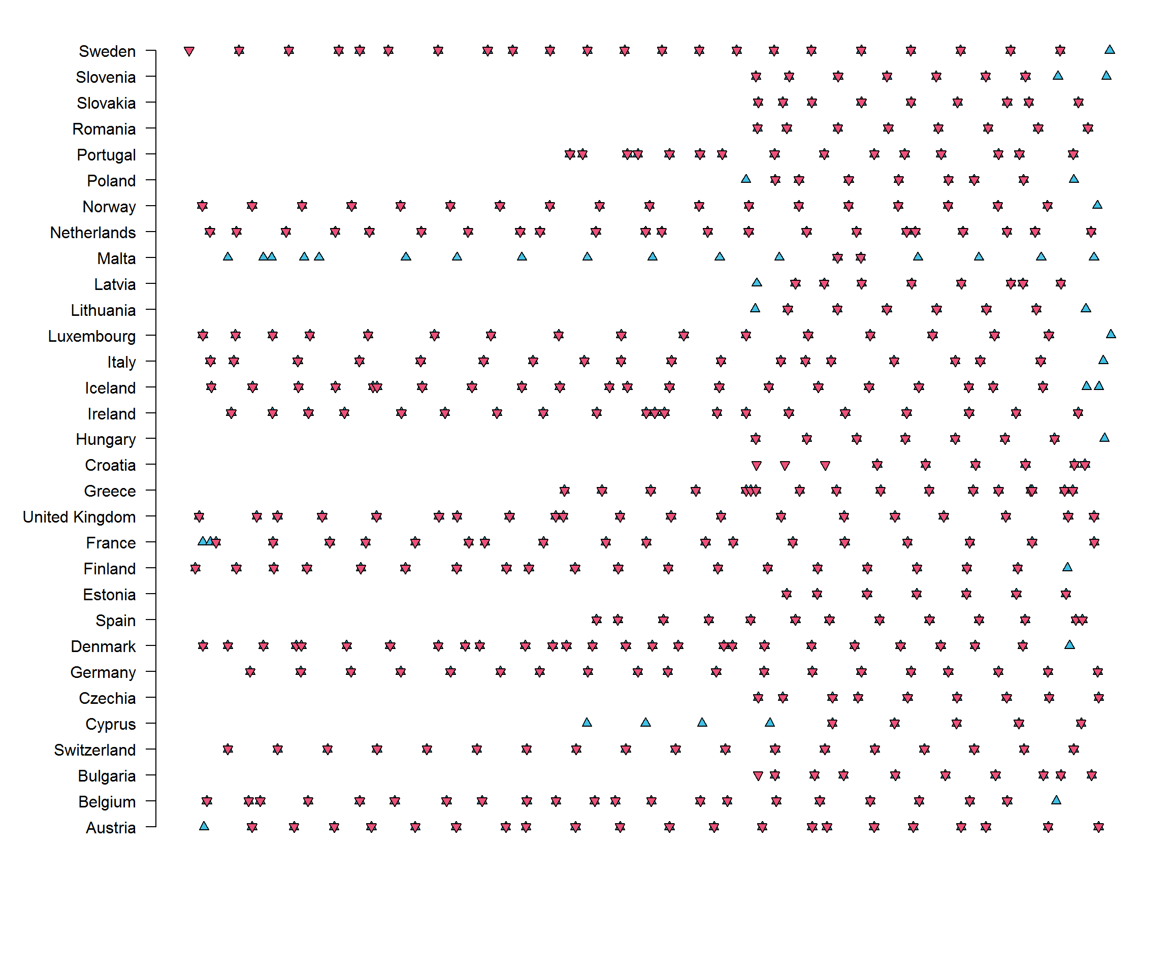
}And we can make a simple plot to show the available election dates in both datasets: ParlGov election dates are in blue triangles and Manifesto election dates are in red triangles. When both are available we see stars.
main.color=rgb(238, 80, 121, alpha=175, max=255)
main.color2=rgb(64,193,230, alpha=175, max=255)
par(mar=c(6,8,1,1))
plot(NULL,type='n',axes=FALSE,ann=FALSE, xlim=c(as.Date('1945-01-01'),as.Date('2019-01-01')), ylim=c(1,31))
#axis(1, at=seq(as.Date('1945-01-01'),as.Date('2019-01-01'),365.25), labels=seq(year(as.Date('1945-01-01')),year(as.Date('2018-01-01')),1), las=2)
axis(2, at=1:length(countries),labels=(countries), las=2 )
for (i in 1:length(countries)){
points(x=cabs$election_date[cabs$country_name==countries[i]], y=rep(i,length(cabs$election_date[cabs$country_name==countries[i]])) , bg=main.color2, pch=24)
points(x=manifestos$edate[manifestos$countryname==countries[i]], y=rep(i,length(manifestos$edate[manifestos$countryname==countries[i]])) , bg=main.color, pch=25)
}
Aligning the party codes
The next preparatory step is to align the party codes so that we can match the two data sources. ParlGov includes the variable cmp that provides the party code as in the Manifesto data. However, there are a lot of missing values. The code below imputes the cmp code to ParlGov whenever possible in order to improve the coverage. First, we can look for cases where the country and party names are exactly the same in both datasets. Second, we apply a list of imputations that I identified from inspecting ‘manually’ the data. Third, we use the newly-released Party Facts dataset that provides some additional matches. (If you notice mistakes or you want to add to the list, you can let me know or directly clone the list on GitHub.)
table(is.na(parties$cmp)) #how many cmp codes are missing? A lot##
## FALSE TRUE
## 412 932#get additional CMP codes if the party names match exactly
parties$cmp2<-parties$cmp #first create a copy of the cmp variable
#for each row in parties, if the cmp code is NA and if the corresponding party name in Manifestos is not NA and the country is the same, record it in cmp2
for (i in 1:nrow(parties)){
if (is.na(parties$cmp)==T)
if (is.na(as.data.frame(manifestos[manifestos$countryname==parties$country_name[i] & manifestos$partyname==parties$party_name_english[i], 'party'][1,]))==T)
next
else
parties$cmp2[i]<-as.data.frame(manifestos[manifestos$countryname==parties$country_name[i] & manifestos$partyname==parties$party_name_english[i], 'party'][1,])
else
next
}
parties$cmp2<-as.numeric(parties$cmp2)
table(is.na(parties$cmp2)) #how many cmp codes are still missing? There is an improvement, but still a lot##
## FALSE TRUE
## 503 841#apply additional imputations of the cmp code
source('cmp code corrections.R')
#source('https://raw.githubusercontent.com/demetriodor/govpositions/master/cmp%20code%20corrections.R')
table(is.na(parties$cmp2)) #there is progress but we can still do better##
## FALSE TRUE
## 545 799#using the newly relased Party Facts data
#get the data
file_name <- "partyfacts-mapping.csv"
url <- "https://partyfacts.herokuapp.com/download/external-parties-csv/"
download.file(url, file_name)
partyfacts <- read_csv(file_name, guess_max = 30000)
#select EU+ countries of interset
partyfacts<-partyfacts %>% filter(country %in% countries.iso)
#subset and join manifesto and parlgov data
dataset_1 <- partyfacts %>% filter(dataset_key == "manifesto")
dataset_2 <- partyfacts %>% filter(dataset_key == "parlgov")
links <- dataset_1 %>% inner_join(dataset_2, by = c("partyfacts_id" = "partyfacts_id"))
links<-links[,c('dataset_party_id.x','dataset_party_id.y')]
colnames(links)<-c('mani','parlgov')
## for some parties, there are more than one Manifesto code for each Parlgov code. Most of these are not missing a cmp code but two parties are.
## (and seven would have been before our custom corrections above)
## We filter so that there is a one-to-one match. As we are not sure which cmp to keep, we just keep the first encountered one
## the code below can be used to inspect these duplicate cases
#temp<-unique(links$parlgov[which(duplicated(links$parlgov)==T)])
#temp2<-parties[is.na(parties$cmp2),]
#temp3<-parties[is.na(parties$cmp),]
#temp[which(temp%in%temp2$party_id==T)]
#temp[which(temp%in%temp3$party_id==T)]
links<-links[!duplicated(links[,c('parlgov')]),]
#merge with the parties data
parties<-merge(parties, links, by.y='parlgov', by.x='party_id', all.x=T)
#if the cmp code is still missing in parties but is not missing in the party facts dataset, impute it
parties$cmp2[is.na(parties$cmp2) & !is.na(parties$mani)]<-parties$mani[is.na(parties$cmp2) & !is.na(parties$mani)]
parties$cmp2<-make.number(parties$cmp2)
table(is.na(parties$cmp2)) #how are we doing? altogether, better (filled in 161 parties in total) but far from perfect match##
## FALSE TRUE
## 573 771Merging the datasets
We made significant progress by imputing missing cmp codes based on different strategies. Again, these are steps that hopefully will become obsolete with future releases of the ParlGov data, but for now they are essential to achieve good match with the Manifesto data. As I will show shortly, we can improve the match even further by identifying some more matches, but first we need to merge the datasets together.
# Merge parties and cabinets
parties$party<-parties$cmp2 #copy the column to use for merge

manipart<-merge(manifestos, parties, by="party") #keep only observations that have CMP codes in ParlGov
manipart$new_id<-paste0(manipart$party_id, ".", manipart$edate) #index variable

cabs$new_id<-paste0(cabs$party_id, '.',cabs$election_date) #index variable
cabinets<-merge(manipart, cabs, by="new_id", all.y=T) #merge parties and cabinets
At this point we can run some additional imputations of Manifesto data. These are mostly cases where Manifesto data exists for a party but not for the exact election. In such cases ParlGov has missing cmp codes, but it is quite reasonable to assign to these parties their positions from other elections close in time (it’s not ideal, but it is better than having no data on these parties at all). Some other cases relate to coalitions where Manifesto data exist only for one of the partners.
# additional cmp imputations
source('more cmp code corrections.R')
#source('https://raw.githubusercontent.com/demetriodor/govpositions/master/more%20cmp%20code%20corrections.R')
We can also create some additional variables that will be useful later on: the seat share of parties and the last date of the cabinet.
cabinets$seats_share <- (cabinets$seats / cabinets$election_seats_total) * 100 #calculate party seat share

#put the end dates of the cabinets in the file, based on the starting date of the next cabinet
for (i in 1:nrow(cabinets)){
  cabinets$end_date[i]<-cabinets$start_date[cabinets$previous_cabinet_id==cabinets$cabinet_id[i] & !is.na(cabinets$previous_cabinet_id)][1]
  }
cabinets$end_date<-as.Date(cabinets$end_date-1)
We can inspect the latest election data availability for each country in both the Manifesto and ParlGov data
# Make table of last elections --------------------------------------------
last.elections<-data.frame(matrix(NA, nrow=length(countries), ncol=3))
colnames(last.elections)<-c('country','manifesto.last','parlgov.last')
for (i in 1:length(countries)){
  last.elections[i,'country']<-countries[i]
  last.elections[i,'manifesto.last']<-(tail(manifestos$edate[manifestos$countryname==countries[i]],1))
  last.elections[i,'parlgov.last']<-(tail(cabs$election_date[cabs$country_name==countries[i]],1))
}
last.elections[,2]<-as.Date(last.elections[,2])
last.elections[,3]<-as.Date(last.elections[,3])
last.elections$same<-ifelse(last.elections[,2]==last.elections[,3], 'same', 'not.same')
last.elections
## country manifesto.last parlgov.last same
## 1 Austria 2017-10-15 2017-10-15 same
## 2 Belgium 2010-06-13 2014-05-25 not.same
## 3 Bulgaria 2017-03-26 2017-03-26 same
## 4 Switzerland 2015-10-18 2015-10-18 same
## 5 Cyprus 2016-05-22 2016-05-22 same
## 6 Czechia 2017-10-21 2017-10-21 same
## 7 Germany 2017-09-24 2017-09-24 same
## 8 Denmark 2011-09-15 2015-06-18 not.same
## 9 Spain 2016-06-26 2016-06-26 same
## 10 Estonia 2015-03-01 2015-03-01 same
## 11 Finland 2011-04-17 2015-04-19 not.same
## 12 France 2017-06-11 2017-06-11 same
## 13 United Kingdom 2017-06-08 2017-06-08 same
## 14 Greece 2015-09-20 2015-09-20 same
## 15 Croatia 2016-09-11 2016-09-11 same
## 16 Hungary 2014-04-06 2018-04-08 not.same
## 17 Ireland 2016-02-26 2016-02-26 same
## 18 Iceland 2013-04-27 2017-10-28 not.same
## 19 Italy 2013-02-24 2018-03-04 not.same
## 20 Luxembourg 2013-10-20 2018-10-14 not.same
## 21 Lithuania 2012-10-14 2016-10-09 not.same
## 22 Latvia 2014-10-04 2014-10-04 same
## 23 Malta 1998-09-05 2017-06-03 not.same
## 24 Netherlands 2017-03-15 2017-03-15 same
## 25 Norway 2013-09-09 2017-09-11 not.same
## 26 Poland 2011-10-09 2015-10-25 not.same
## 27 Portugal 2015-10-04 2015-10-04 same
## 28 Romania 2016-12-11 2016-12-11 same
## 29 Slovakia 2016-03-05 2016-03-05 same
## 30 Slovenia 2011-12-04 2018-06-03 not.same
## 31 Sweden 2014-09-14 2018-09-09 not.sameWe can inspect the share of missing Manifesto data for the subset of parties in cabinet, and we can do that per cabinet (output not shown).
### this code computes the seat shares of parties that do  and do not have corresponding cmp codes
m.data = cabinets%>% group_by(cabinet_id) %>% summarise(country=country_name.y[1], election.date=election_date[1],
                                                   start.date = start_date[1], end.date = end_date[1],
                                                   caretaker = caretaker[1],
                                                   seat.share = round(sum.na(seats_share),0),
                                                   seat.share.valid = round(sum.na(seats_share[!is.na(cmp2)]),0),
                                                   seat.share.missing = round(sum.na(seats_share[is.na(cmp2)]),0))
m.data$share.missing<-round(m.data$seat.share.missing/m.data$seat.share*100,0)
m.data<-m.data[order(m.data$country, m.data$election.date),]
head(m.data)
## # A tibble: 6 x 10
## cabinet_id country election.date start.date end.date caretaker
## <int> <chr> <date> <date> <date> <int>
## 1 133 Austria 1945-11-25 1945-12-04 1947-11-19 0
## 2 884 Austria 1945-11-25 1947-11-20 1949-11-07 0
## 3 560 Austria 1949-10-09 1952-10-28 1953-04-01 1
## 4 775 Austria 1949-10-09 1949-11-08 1952-10-27 0
## 5 659 Austria 1953-02-22 1953-04-02 1956-06-28 0
## 6 105 Austria 1956-05-13 1956-06-29 1959-07-15 0
## # ... with 4 more variables: seat.share <dbl>, seat.share.valid <dbl>,
## # seat.share.missing <dbl>, share.missing <dbl>m.data$end.date2<-as.Date(ifelse(is.na(m.data$end.date)==T, 17896, m.data$end.date)) #assign date of data collection as end date for cabinets with missing end dates
#there are some cabinets, mostly in France and Monti in Italy for which the seat share sums up to more than 100%We can also produce a graph that shows the share of missing data for parties in cabinet: the rectangles below show each cabinet per country (since 1990) and are colored in solid black if Manifesto data is available for 100% of the parties in the cabinet and white if no data is available, with darker shades of grey corresponding to higher shares of available data (the ‘c’ letter stands for caretaker cabinets). The figure shows that for those cabinets for which Manifesto data is in principle available (the election manifestos have been coded), the share of cabinet parties included in the combined dataset is typically 100% or close to that (with the exception of some caretaker cabinets, which are often run by experts and not parties).
cols<-colorRampPalette(c("black", "white"))(10)
m.data$share.missing<-cut(m.data$share.missing, breaks=c(-Inf,10,20,30,40,50,60,70,80,90,100), labels=seq(1,10,1))
m.data$color<-cols[m.data$share.missing]
m.data$color<-ifelse(is.na(m.data$color),0,m.data$color)
par(mar=c(6,8,1,1))
plot(NULL, xlim=c(as.Date('1990-01-01'),as.Date('2019-01-01')), ylim=c(1,31), axes = F, ann=T, xlab='', ylab='')
axis(1, at=seq(as.Date('1990-01-01'),as.Date('2019-01-01'),365.25), labels=seq(year(as.Date('1990-01-01')),year(as.Date('2018-01-01')),1), las=2)
axis(2, at=1:length(countries),labels=(countries), las=2 )
for (i in 1:nrow(m.data)){
rect(xlef = m.data$start.date[i], xright = m.data$end.date2[i], ytop = which(countries==m.data$country[i])+0.3, ybottom = which(countries==m.data$country[i])-0.3, border='red', col=m.data$color[i])
points(x=m.data$start.date[i]+70, y=which(countries==m.data$country[i]), pch='c', cex=0.8, col=ifelse(m.data$caretaker[i]==1, 'red',rgb(64,193,230, alpha=0, max=255)))
}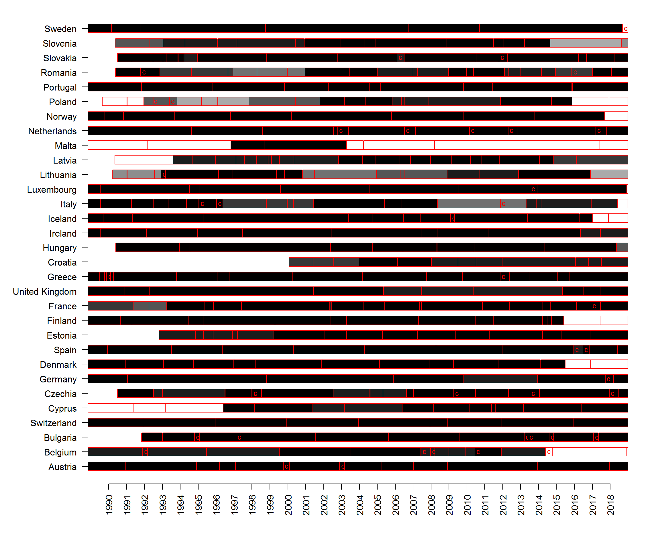 We should assign 31 December 2018, the day when I last obtained the data, as the end day of the cabinets for which this day is not recorded. This will simplify the code for calculating the positions significantly, as we will not have to deal with NAs in the ‘end date’ column.
cabinets$end_date<-as.Date(ifelse(is.na(cabinets$end_date), as.Date('2018-12-31', "%Y-%m-%d"),cabinets$end_date ))Because we imputed some Manifesto data to the ParlGov files based on the party identity, sometimes disregarding the exact election for which the manifestos were coded, there are some cases where we now have data for parties and elections for which manifestos have not been actually coded. We might want to set these observations back to NA.
#after the imputation, some parties have positions for elections for which manifesto data has not been collected
for (i in 1:nrow(cabinets)){
  if (!is.na(cabinets$cmp2[i]) & cabinets$election_date[i] > last.elections$manifesto.last[last.elections$country==cabinets$country_name.y[i]])
    print (cabinets[i,179:196])
  else
    next
}
#we might want to excluded these parties
#affects 4 government parties, 2 in hungary and 2 in Slovenia (one party, two cabinets)
for (i in 1:nrow(cabinets)){
  if (!is.na(cabinets$cmp2[i]) & cabinets$election_date[i] > last.elections$manifesto.last[last.elections$country==cabinets$country_name.y[i]])
    cabinets[i,1:174]<-NA
  else
    next
}
At this point it’s a good idea to save the resulting dataset so that it can be retrieved directly later.
#write.csv (cabinets, 'cabinets2019.csv') #save the resulting file
#cabinets<-read.csv ('cabinets2019.csv', as.is=TRUE) #uncomment if you want to load the file directly once you have saved it

#save(cabinets, file = "cabinets2019.RData")# save in RData format
#load("cabinets2019.RData") # to load the data
All the code for data preparation, aligning and merging the datasets is collected here:
#source('https://raw.githubusercontent.com/demetriodor/govpositions/master/data_preparation_code.R')Computing new party positions
That was all just preparatory work to get a dataset that combines the Manifesto and ParlGov data, inspects the resulting data and creates some new variables. Now we are ready to get down to the real business and start computing party and government positions from the data.
The Manifesto Corpus data already includes predefined scales of party positions : rile (Right-left), planeco, markeco, welfare, intpeace (for details, see the Manifesto Corpus codebook). But we might want to create our own scales by combining individual content items (per101-706; per1011-7062; per103_1-703_2), which track the ‘share of quasi-sentences in the respective category calculated as a fraction of the overall number of allocated codes per document’. Some of these items can load positively on the scale, and some can load negatively.
Here is a function that computes party positions on new scales defined by the user. The function takes as arguments two vectors: ‘x’ for items that load positively on the scale and ‘y’ for items that load negatively. The vectors can be of length 1, i.e. only one item can be provided, or longer. Each of the two vectors can be skipped (if we do not have items that load either positively or negatively), but at least one of the two needs to be provided (otherwise, we have nothing to compute). The function will return NA for each case (party) for which no item has valid values, but will ignore NAs if at least one valid value is present. We can also specify explicitly the dataset from which the positions are to be computed. By default this is called ‘cabinets’, so unless you specify something else, this is where the function will look for the variables.
pos.add<-function (x=NA,y=NA, data=cabinets) {
  pos = if (is.na(y[1]))
    rowsum.allna(data[, x, drop=F])
  else if (is.na(x[1]))
    -rowsum.allna(data[, y, drop=F])
  else
    rowsum.allna(data[, x, drop=F])-rowsum.allna(data[, y, drop=F])
  pos
}
To illustrate how the function works, we create a new ‘nationalism’ scale, which adds positive mentions of ‘National way of life’ (per601) and subtracts negative mentions of the ‘National way of life’ (per602). The function can also be used for the existing scales, which will come in handy. The third example shows that we can point to a different dataset, as long as it is available in the environment and contains the variables we need. This function is kept simple on purpose, so there are not further arguments to pass, such as start and end date or country. And the output is just a vector of numbers. Below we will embed this (and other) simple functions into a wrapper that can do all that.
nationalism<-pos.add(x='per601',y='per602') #new scale of two items, one loading positively and one negatively
cbind(nationalism[1:3], cabinets[1:3, c('per601','per602')]) #check that it works as intended
## nationalism[1:3] per601 per602
## 1 1.604 2.139 0.535
## 2 1.604 2.139 0.535
## 3 NA NA NArile<-pos.add(x='rile') #does it work to retrieve a predefined scale?
which(rile!=cabinets$rile) #yes, it does, no unmatched values## integer(0)conserv<-pos.add(x=c('per601','per603','per605'),y=c('per602','per604'), data=manifestos) #new scale of several items, some loading positively and some negatively
cbind(conserv[1:5], manifestos[1:5, c('per601','per603','per605','per602', 'per604')]) #check that it works as intended## conserv[1:5] per601 per603 per605 per602 per604
## 1 0.000 0.000 0.0 0 0 0
## 2 0.000 0.000 0.0 0 0 0
## 3 6.400 0.000 6.4 0 0 0
## 4 14.000 3.500 10.5 0 0 0
## 5 4.762 4.762 0.0 0 0 0The function above computes the shares of statements (quasi-sentences) from the party manifestos that fit each topic (item). Sometimes, we might be interested in the actual number of statement instead. To do that we only need some minor modifications of the function:
pos.add.n<-function (x=NA,y=NA, data=cabinets) {
  pos = if (is.na(y[1]))
    round(rowsum.allna(data[,x, drop=F])*data[,'total']/100)
  else if (is.na(x[1]))
    -round(rowsum.allna(data[,y, drop=F])*data[,'total']/100)
  else
    round(rowsum.allna(data[,x, drop=F])*data[,'total']/100) - round(rowsum.allna(data[,y, drop=F])*data[,'total']/100)
  pos
}

nationalism2<-pos.add.n(x='per601',y='per602') #new scale of two items in raw numbers, one loading positively and one negatively
cbind(nationalism2[1:3], cabinets[1:3, c('per601','per602', 'total')]) #check that it works as intended
## nationalism2[1:3] per601 per602 total
## 1 3 2.139 0.535 187
## 2 3 2.139 0.535 187
## 3 NA NA NA NAWe can also implement the approach to calculating scales from Manifesto items introduced by Lowe, Benoit, Mikhaylov, and Laver (2011). This approach takes the difference between the natural logarithm of the number of positively-loading statements plus 0.5 and the natural logarithm of the number of negatively-loading statements plus 0.5.
pos.lbml<-function (x=NA,y=NA, data=cabinets) {
  pos = if (is.na(y[1]))
    log (round(rowsum.allna(data[, x, drop=F])*data[, 'total']/100) + 0.5) - log (0.5)
  else if (is.na(x[1]))
    - log (round(rowsum.allna(data[, y, drop=F])*data[, 'total']/100) + 0.5) + log (0.5)

  else
    log((round(rowsum.allna(data[, x, drop=F])*data[, 'total']/100) + 0.5)) - log((round(rowsum.allna(data[, y, drop=F])*data[, 'total']/100) + 0.5))
  pos
}
Let’s see the function in action.
nationalism<-pos.lbml(x='per601',y='per602') #new scale of two items, one loading positively and one negatively, based on the Lowe et al. (2011) approach
cbind(nationalism[1:3], cabinets[1:3, c('per601','per602', 'total')]) #check that it worls as intended
## nationalism[1:3] per601 per602 total
## 1 1.098612 2.139 0.535 187
## 2 1.098612 2.139 0.535 187
## 3 NA NA NA NAlog(round(2.139*187/100,0)+0.5)-log(round(0.535*187/100,0)+0.5) #check that it matches a manual calculation## [1] 1.098612There is another way to calculate party positions, proposed by Kim and Fording (2002), which is essentially the difference between the positive and negative statements divided by their sum. Here it is implemented in a function:
pos.kf<-function (x=NA,y=NA, data=cabinets) {
  pos = (round(rowsum.allna(data[,x, drop=F])*data[,'total']/100) - round(rowsum.allna(data[,y, drop=F])*data[,'total']/100))/
    (round(rowsum.allna(data[,x, drop=F])*data[,'total']/100) + round(rowsum.allna(data[,y, drop=F])*data[,'total']/100))
  pos
}

nationalism3<-pos.kf(x='per601',y='per602') #new scale of two items in raw numbers, one loading positively and one negatively
cbind(nationalism3[1:3], cabinets[1:3, c('per601','per602', 'total')]) #check that it works as intended
## nationalism3[1:3] per601 per602 total
## 1 0.6 2.139 0.535 187
## 2 0.6 2.139 0.535 187
## 3 NA NA NA NAThe functions above compute positions that are composed of items that might load positively or negatively. The Manifesto Corpus data can also be used to estimate the salience of topics (it’s actually better suited to do that than to estimate positions as such.) Therefore, we can define modifications of the functions above that compute salience. Now the functions take only one argument (‘x’) rather than two (‘x’ and ‘y’), so put all the items that load on the scale there (if an ‘y’ argument is provided it will be ignored but it will not return an error). Lowe et al. (2011) also suggest a measure of policy importance (salience) that we can implement as a function as well.
pos.add.sal<-function (x=NA, ..., data=cabinets) {
  pos = rowsum.allna(data[, x, drop=F])
  pos
}

pos.add.n.sal<-function (x=NA, ..., data=cabinets) {
  pos = round(rowsum.allna(data[,x, drop=F])*data[,'total']/100)
  pos
}

pos.lbml.sal<-function (x=NA, ..., data=cabinets) {
  pos = log((round(rowsum.allna(data[, x, drop=F])*data[, 'total']/100) + 1)/ data[, 'total'])
  pos
}
Let’s check whether it works.
head(pos.add.sal(x=c('per601', 'per602')))## [1] 2.674 2.674 NA NA NA NAhead(pos.add.n.sal(x='per601', y='per602')) #y isignored## [1] 4 4 NA NA NA NAhead(pos.lbml.sal(x=c('per601', 'per602'), data=manifestos) ) #differnt data than the default## total
## 1 -3.951244
## 2 -4.499810
## 3 -4.143135
## 4 -2.944439
## 5 -2.351375
## 6 -3.912023Wrapping up the party position functions
Having defined these basic functions that calculate party-level positions and salience, we can wrap them up into another function that takes more arguments and customizes the output. In addition to the ‘x’,‘y’ and ‘data’ arguments, this new function takes the method of calculation as an argument. The ‘method’ can be any of the functions defined above: pos.add (default), pos.add.n, pos.lbml, pos.add.sal, pos.add.n.sal, pos.lbml.sal. We can also specify a name for the output variable (‘position’ is the default). We can specify the type of output we want: a vector of numbers (‘vector’), the original data table with the new position variable attached (‘attach’) or a small new table with the country, party name, election date and the values of the position variable (‘table’, which is the default). We can also specify start and end dates that are of interest, as well as a subset of countries. If we specify a different dataset than the default ‘cabinets’, we also need to specify the names of the variables in that dataset that contain the start and end dates, and the country and party names. Be careful: when the requested output is a vector, it is assigned to the global environment with the specified name.
party.pos<-function (x=NA,y=NA, data=cabinets, method = pos.add, name = 'position', output = 'table', start='1945-01-01', end='2018-12-31', countries=countries.list, start_col='election_date', end_col='election_date', country_col='country_name.y', party_col='partyname') {
  data<-data.frame(data)
  dataset<- data%>%filter(data[,start_col] >= start & data[,end_col] <= end & data[,country_col]%in%countries) #filter for the required time and geo scope
  temp = method (x,y, data=dataset) #run the party position calculation function

  if (output=='vector'){
    assign(name, temp, envir = .GlobalEnv)
    return (temp)}
  else if (output=='attach'){
    data.out<-cbind(dataset, temp)
    colnames(data.out)[ncol(data.out)]<-name
    return(data.out)}
  else if (output=='table'){
    data.out<-cbind(dataset, temp)
    data.out = data.out[,c(country_col, start_col, party_col, 'temp')]
    colnames(data.out)[1:4]<-c('country','election.date', 'party.name', name)
    return(data.out)}
  }
Here are examples how the function works with different settings of the attributes.
tail(party.pos (x='per601', y='per602', countries='Austria'))## country election.date party.name position
## 131 Austria 2002-11-24 Austrian Social Democratic Party 0.695
## 132 Austria 2006-10-01 Austrian Social Democratic Party 1.803
## 133 Austria 2008-09-28 Austrian Social Democratic Party 1.912
## 134 Austria 2013-09-29 Austrian Social Democratic Party 0.690
## 135 Austria 2013-09-29 Austrian Social Democratic Party 0.690
## 136 Austria 2017-10-15 Austrian Social Democratic Party 1.799party.pos (x='per601', y='per602', start='2000-01-01', method=pos.lbml, name='nationalism', end='2010-12-31', countries='Sweden')## country election.date party.name nationalism
## 1 Sweden 2002-09-15 Green Ecology Party 0.000000
## 2 Sweden 2006-09-17 Green Ecology Party 0.000000
## 3 Sweden 2010-09-19 Green Ecology Party 0.000000
## 4 Sweden 2002-09-15 Centre Party 0.000000
## 5 Sweden 2006-09-17 Centre Party 1.945910
## 6 Sweden 2010-09-19 Centre Party 0.000000
## 7 Sweden 2010-09-19 Sweden Democrats 3.931826
## 8 Sweden 2002-09-15 Christian Democrats 0.000000
## 9 Sweden 2006-09-17 Christian Democrats 1.945910
## 10 Sweden 2010-09-19 Christian Democrats 0.000000
## 11 Sweden 2002-09-15 Moderate Coalition Party 1.098612
## 12 Sweden 2006-09-17 Moderate Coalition Party 2.197225
## 13 Sweden 2010-09-19 Moderate Coalition Party 2.944439
## 14 Sweden 2002-09-15 Left Party 0.000000
## 15 Sweden 2006-09-17 Left Party 0.000000
## 16 Sweden 2010-09-19 Left Party 1.098612
## 17 Sweden 2002-09-15 Liberal Peoples Party 1.098612
## 18 Sweden 2006-09-17 Liberal Peoples Party 2.564949
## 19 Sweden 2010-09-19 Liberal Peoples Party 2.708050
## 20 Sweden 2002-09-15 Social Democratic Labour Party 0.000000
## 21 Sweden 2006-09-17 Social Democratic Labour Party 3.135494
## 22 Sweden 2010-09-19 Social Democratic Labour Party 0.000000party.pos (x=c('per601', 'per603'), y=c('per602', 'per604'), start='1995-01-01', method=pos.lbml, name='nationalism', end='2000-12-31', countries='Denmark',
data=manifestos, start_col='edate', end_col='edate', country_col='countryname', party_col='partyname')## country election.date party.name nationalism
## 1 Denmark 1998-03-11 Red-Green Unity List 0.000000
## 2 Denmark 1998-03-11 Socialist Peoples Party 1.098612
## 3 Denmark 1998-03-11 Social Democratic Party 2.512306
## 4 Denmark 1998-03-11 Centre Democrats -1.098612
## 5 Denmark 1998-03-11 Danish Social-Liberal Party 0.000000
## 6 Denmark 1998-03-11 Liberals 0.000000
## 7 Denmark 1998-03-11 Christian Peoples Party 4.110874
## 8 Denmark 1998-03-11 Conservative Peoples Party 3.218876
## 9 Denmark 1998-03-11 Danish Peoples Party 1.098612
## 10 Denmark 1998-03-11 Progress Party 1.945910party.pos (x='per601', y='per602', countries=c('Germany'), start='2010-01-01', end='2014-01-01', method=pos.add.n.sal, name='nat', output='vector')## [1] 68 29 17 NAnat## [1] 68 29 17 NAd<-party.pos (x='per601', y='per602', countries=c('Germany','France'), start='2010-01-01', method=pos.add.n.sal, name='nat', output='attach')
d[70:75, 192:197]## cabinet_party seats election_seats_total seats_share end_date nat
## 70 0 69 709 9.732017 2018-12-31 NA
## 71 1 17 577 2.946274 2014-03-30 1
## 72 1 17 577 2.946274 2017-06-13 1
## 73 0 17 577 2.946274 2016-02-10 1
## 74 1 17 577 2.946274 2016-12-05 1
## 75 0 17 577 2.946274 2017-06-20 1Aggregating party positions into government positions
We are finally ready to compute government (cabinet) positions from the party-level data. There are different ways to do that. Two popular ones are (1) to take the simple mean of the positions of all cabinet parties or (2) to weigh each cabinet party positions by its share of seats relative to the seats of all cabinet parties. In the function, we will implement both these methods. Also, we will provide the minimum and maximum position on the created scale, as well as the range between the two. All of these measures are useful for working with government positions in empirical research. If you need additional ones, let me know or you can directly adapt the code. The function also returns the number of parties in each government and the seat share of governing parties (from the total seat share of all governing parties) for which there is valid data on the requested positions.
The function to compute government positions takes many of the arguments that the party computation functions do. But since we need a dataset that contains both party positions and government data, such as duration and seat shares, we assume that the functions should only work on the ‘cabinets’ dataset as constructed above. The output is always a small table.
gov.pos<-function (x=NA,y=NA, data=cabinets, method = pos.add, name ='position', start='1945-01-01', end='2018-12-31', countries=countries.list) {

  dataset2 = party.pos(x=x, y=y, data=data, method=method, output='attach') #calculate the party score and attach to the dataframe
  colnames(dataset2)[ncol(dataset2)]<-'party.score' #rename the last column temporarity

  dataset2<- dataset2%>%
    filter(election_date > start & election_date < end & country_name.y%in%countries & cabinet_party==1)%>%
    select(cabinet_id, seats_share,country_name.y,start_date,end_date,election_date, party.score)

  #first, create a variable that calculates the party seats share from all parties in government *that have a valid position*
  for (i in unique(dataset2$cabinet_id)){
    dataset2[dataset2$cabinet_id==i,'rel_seats_share'] = dataset2[dataset2$cabinet_id==i,'seats_share'] / sum.allna(dataset2[dataset2$cabinet_id==i & !is.na(dataset2$party.score),'seats_share'])
  }

  #now aggregate per cabinet
  m = dataset2%>% group_by(cabinet_id) %>% summarise(country=country_name.y[1], election.date=election_date[1],
                                                     start.date = start_date[1], end.date = end_date[1],
                                                     simple.mean  = round(mean.allna(party.score),2),
                                                     weighted.mean = round(weighted.mean(party.score, rel_seats_share, na.rm=T),2),
                                                     minimum = round(min.allna(party.score),2),
                                                     maximum = round(max.allna(party.score),2),
                                                     range = abs (round(max.allna(party.score),2) -round(min.allna(party.score),2)),
                                                     parties.number = n(),
                                                     share.missing = round(sum.na(seats_share[is.na(party.score)])/sum.na(seats_share)*100,0)
  )
  m<-m[order(m$country, m$start.date),]
  m
}

#examples
data.frame(tail(gov.pos (x='per601', y='per602', countries='Austria')))
## cabinet_id country election.date start.date end.date simple.mean
## 1 888 Austria 2002-11-24 2005-04-05 2007-01-10 1.98
## 2 583 Austria 2006-10-01 2007-01-11 2008-12-01 3.74
## 3 268 Austria 2008-09-28 2008-12-02 2013-12-15 3.00
## 4 1070 Austria 2013-09-29 2013-12-16 2016-05-16 0.90
## 5 1485 Austria 2013-09-29 2016-05-17 2017-12-17 0.90
## 6 1521 Austria 2017-10-15 2017-12-18 2018-12-31 4.31
## weighted.mean minimum maximum range parties.number share.missing
## 1 0.79 0.37 3.58 3.21 2 0
## 2 3.71 1.80 5.68 3.88 2 0
## 3 2.94 1.91 4.10 2.19 2 0
## 4 0.89 0.69 1.12 0.43 2 0
## 5 0.89 0.69 1.12 0.43 2 0
## 6 4.17 2.86 5.75 2.89 2 0data.frame(gov.pos (x='per601', y='per602', start='2000-01-01', method=pos.lbml, name='nationalism', end='2010-12-31', countries='Sweden'))## cabinet_id country election.date start.date end.date simple.mean
## 1 641 Sweden 2002-09-15 2002-10-21 2006-10-04 0.00
## 2 475 Sweden 2006-09-17 2006-10-05 2010-09-18 2.16
## 3 854 Sweden 2010-09-19 2010-09-19 2014-10-01 1.41
## weighted.mean minimum maximum range parties.number share.missing
## 1 0.00 0.00 0.00 0.00 1 0
## 2 2.18 1.95 2.56 0.61 4 0
## 3 2.20 0.00 2.94 2.94 4 0Aggregating government positions into time series
For many application we need the government position data to be in the form of time series. The function below takes the government positions and returns a table in which the positions are recorded for each month (between requested start and end dates) and each country. The output can also be aggregated per year instead of per month. In that case the yearly values are the means of the month values for the particular year. Whether monthly or yearly data is desired can be specified by the argument ‘time’ (with ‘month’ as the default).
gov.pos.time <-function (x=NA,y=NA, data=cabinets, method = pos.add, name ='position', start='1945-01-01', end='2018-12-31', countries=countries.list, time='month') {

  dat<-gov.pos (x=x,y=y, data=data, method=method, countries=countries,start='1945-01-01', end='2018-12-31')
  dat$startY<-year(dat$start.date)
  dat$startYM<-as.yearmon(dat$start.date)
  dat$endY<-year(dat$end.date)
  dat$endYM<-as.yearmon(dat$end.date)

  u.c<-countries
  u.m<-as.yearmon(seq.Date(from=as.Date(start), to=as.Date(end), by='month'))

  month.table<-expand.grid(u.c, u.m)
  colnames(month.table)<-c('country','month.year')
  month.table$simple.mean<-NA
  month.table$weighted.mean<-NA
  month.table$minimum<-NA
  month.table$maximum<-NA
  month.table$range<-NA
  month.table$parties.number<-NA
  month.table$share.missing<-NA


  for (i in 1:nrow(month.table)){
    try(month.table[i, 3:9] <-dat[which(dat$country==month.table$country[i] & dat$startYM <= month.table$month.year[i] & dat$endYM > month.table$month.year[i]), 6:12], silent=TRUE)
  }
  month.table<-month.table[order(month.table$country, month.table$month.year),]

  if (time=='month'){
    return (month.table)}
  else if (time=='year'){
    month.table$year<-year(month.table$month.year)
    month.table$index<-paste0(month.table$country, '.', month.table$year)
    year.table = month.table%>% group_by(index) %>% summarise(country=country[1], year= year[1],
                                                              simple.mean = mean.allna(simple.mean),
                                                              weighted.mean = mean.allna(weighted.mean),
                                                              minimum = mean.allna(minimum),
                                                              maximum = mean.allna(maximum),
                                                              range = mean.allna(range),
                                                              parties.number = mean.allna(parties.number),
                                                              share.missing = mean.allna(share.missing))
    return (year.table)
    }
  }
And examples:
tail(gov.pos.time (x='per601', y='per602', start='2000-01-01', end='2010-01-06', countries='Austria'))## country month.year simple.mean weighted.mean minimum maximum range
## 116 Austria Aug 2009 3 2.94 1.91 4.1 2.19
## 117 Austria Sep 2009 3 2.94 1.91 4.1 2.19
## 118 Austria Oct 2009 3 2.94 1.91 4.1 2.19
## 119 Austria Nov 2009 3 2.94 1.91 4.1 2.19
## 120 Austria Dec 2009 3 2.94 1.91 4.1 2.19
## 121 Austria Jan 2010 3 2.94 1.91 4.1 2.19
## parties.number share.missing
## 116 2 0
## 117 2 0
## 118 2 0
## 119 2 0
## 120 2 0
## 121 2 0gov.pos.time (x=c('per601', 'per603'), y='per602', method=pos.lbml, start='1990-01-01', end='2010-12-31', countries='Sweden', time='year')## # A tibble: 21 x 10
## index country year simple.mean weighted.mean minimum maximum range
## <chr> <fct> <dbl> <dbl> <dbl> <dbl> <dbl> <dbl>
## 1 Swed~ Sweden 1990 0 0 0 0 0
## 2 Swed~ Sweden 1991 0.495 0.562 0.275 0.735 0.46
## 3 Swed~ Sweden 1992 1.98 2.25 1.1 2.94 1.84
## 4 Swed~ Sweden 1993 1.98 2.25 1.1 2.94 1.84
## 5 Swed~ Sweden 1994 1.97 2.17 1.31 2.69 1.38
## 6 Swed~ Sweden 1995 1.95 1.95 1.95 1.95 0
## 7 Swed~ Sweden 1996 1.95 1.95 1.95 1.95 0
## 8 Swed~ Sweden 1997 1.95 1.95 1.95 1.95 0
## 9 Swed~ Sweden 1998 1.74 1.74 1.74 1.74 0
## 10 Swed~ Sweden 1999 1.1 1.1 1.1 1.1 0
## # ... with 11 more rows, and 2 more variables: parties.number <dbl>,
## # share.missing <dbl>gov.pos.time (x=c('per601', 'per603'), y='per602', method=pos.add.n.sal, start='1990-01-01', end='2010-12-31', countries='Netherlands', time='year')## # A tibble: 21 x 10
## index country year simple.mean weighted.mean minimum maximum range
## <chr> <fct> <dbl> <dbl> <dbl> <dbl> <dbl> <dbl>
## 1 Neth~ Nether~ 1990 28 29.3 2 54 52
## 2 Neth~ Nether~ 1991 28 29.3 2 54 52
## 3 Neth~ Nether~ 1992 28 29.3 2 54 52
## 4 Neth~ Nether~ 1993 28 29.3 2 54 52
## 5 Neth~ Nether~ 1994 23.8 25.6 1.58 49.8 48.2
## 6 Neth~ Nether~ 1995 18 20.4 1 44 43
## 7 Neth~ Nether~ 1996 18 20.4 1 44 43
## 8 Neth~ Nether~ 1997 18 20.4 1 44 43
## 9 Neth~ Nether~ 1998 15.9 16.9 4.33 32.8 28.4
## 10 Neth~ Nether~ 1999 13 12.0 9 17 8
## # ... with 11 more rows, and 2 more variables: parties.number <dbl>,
## # share.missing <dbl>We can source all the functions together from these two files: one for the party-level functions and one for the aggregations per government and over time.
Source all functions together
These two files collect all functions so that we can source them directly from local files or from the web (GitHub). The first file collects the party-level functions and the second file contains the aggregation functions per government (caibnet) and over time.
#source('party.position.functions.r')
#source('https://raw.githubusercontent.com/demetriodor/govpositions/master/party_position_functions.R')
#source('government.position.functions.r')
#source('https://raw.githubusercontent.com/demetriodor/govpositions/master/government_position_functions.R')
References
Here is again a link to the GitHub repository of the project. You are welcome to contribute.
You can reach me on Twitter (@DToshkov) or send me an email. If you use these functions, you can cite them as:
- Toshkov, Dimiter. 2019. ‘R functions for calculating party positions and aggregating government positions from the Manifesto Corpus data wtih ParlGov’. link
Here are the references for the datasets used and the stuides referenced in this tutorial:
Döring, Holger and Philip Manow. 2018. Parliaments and Governments Database (ParlGov): Information on Parties, Elections and Cabinets in Modern Democracies.
Döring, Holger, and Sven Regel. 2019. “Party Facts: A Database of Political Parties Worldwide.” Party Politics, Early View.
Kim, Heemin, and Richard Fording. 2002. “Government Partisanship in Western Democracies, 1945-1998.” European Journal of Political Research 41: 187-202.
Krause, Werner, Lehmann, Pola, Lewandowski, Jirka, Matthieß, Theres, Merz, Nicolas, Regel, Sven. 2018. “Manifesto Corpus. Version: 2018-2.” Berlin: WZB Berlin Social Science Center.
Lowe, Will, Kenneth Benoit, Slava Mikhaylov, and Michael Laver. 2011. “Scaling Policy Preferences from Coded Political Texts.” Legislative Studies Quarterly 36 (1): 123-55. doi:10.1111/j.1939-9162.2010.00006.x.
Volkens, Andrea, Krause, Werner, Lehmann, Pola, Matthieß, Theres, Merz, Nicolas, Regel, Sven, Weßels, Bernhard. 2018. “The Manifesto Data Collection. Manifesto Project (MRG/CMP/MARPOR). Version 2018b.” Berlin: Wissenschaftszentrum Berlin für Sozialforschung (WZB). https://doi.org/10.25522/manifesto.mpds.2018b
The End
session_info()## - Session info ----------------------------------------------------------
## setting value
## version R version 3.5.1 (2018-07-02)
## os Windows 7 x64
## system x86_64, mingw32
## ui RTerm
## language (EN)
## collate English_United States.1252
## ctype English_United States.1252
## tz Europe/Berlin
## date 2019-01-30
##
## - Packages --------------------------------------------------------------
## package * version date lib source
## assertthat 0.2.0 2017-04-11 [1] CRAN (R 3.5.1)
## backports 1.1.2 2017-12-13 [1] CRAN (R 3.5.0)
## base64enc 0.1-3 2015-07-28 [1] CRAN (R 3.5.0)
## bindr 0.1.1 2018-03-13 [1] CRAN (R 3.5.1)
## bindrcpp * 0.2.2 2018-03-29 [1] CRAN (R 3.5.1)
## callr 3.0.0 2018-08-24 [1] CRAN (R 3.5.1)
## cli 1.0.1 2018-09-25 [1] CRAN (R 3.5.1)
## countrycode * 1.1.0 2018-10-27 [1] CRAN (R 3.5.1)
## crayon 1.3.4 2017-09-16 [1] CRAN (R 3.5.1)
## curl 3.2 2018-03-28 [1] CRAN (R 3.5.1)
## desc 1.2.0 2018-05-01 [1] CRAN (R 3.5.1)
## devtools * 2.0.1 2018-10-26 [1] CRAN (R 3.5.1)
## digest 0.6.18 2018-10-10 [1] CRAN (R 3.5.1)
## dplyr * 0.7.7 2018-10-16 [1] CRAN (R 3.5.1)
## DT 0.5 2018-11-05 [1] CRAN (R 3.5.2)
## evaluate 0.12 2018-10-09 [1] CRAN (R 3.5.1)
## fansi 0.4.0 2018-10-05 [1] CRAN (R 3.5.1)
## foreign 0.8-70 2017-11-28 [1] CRAN (R 3.5.1)
## fs 1.2.6 2018-08-23 [1] CRAN (R 3.5.1)
## functional 0.6 2014-07-16 [1] CRAN (R 3.5.2)
## glue 1.3.0 2018-07-17 [1] CRAN (R 3.5.1)
## hms 0.4.2 2018-03-10 [1] CRAN (R 3.5.1)
## htmltools 0.3.6 2017-04-28 [1] CRAN (R 3.5.1)
## htmlwidgets 1.3 2018-09-30 [1] CRAN (R 3.5.1)
## httr 1.3.1 2017-08-20 [1] CRAN (R 3.5.1)
## install.load * 1.2.1 2016-07-12 [1] CRAN (R 3.5.2)
## jsonlite 1.5 2017-06-01 [1] CRAN (R 3.5.1)
## knitr 1.20 2018-02-20 [1] CRAN (R 3.5.1)
## lattice 0.20-35 2017-03-25 [1] CRAN (R 3.5.1)
## lubridate * 1.7.4 2018-04-11 [1] CRAN (R 3.5.1)
## magrittr 1.5 2014-11-22 [1] CRAN (R 3.5.1)
## manifestoR * 1.3.0 2018-05-28 [1] CRAN (R 3.5.2)
## memoise 1.1.0 2017-04-21 [1] CRAN (R 3.5.1)
## mnormt 1.5-5 2016-10-15 [1] CRAN (R 3.5.0)
## nlme 3.1-137 2018-04-07 [1] CRAN (R 3.5.1)
## NLP * 0.2-0 2018-10-18 [1] CRAN (R 3.5.2)
## pillar 1.3.0 2018-07-14 [1] CRAN (R 3.5.1)
## pkgbuild 1.0.2 2018-10-16 [1] CRAN (R 3.5.1)
## pkgconfig 2.0.2 2018-08-16 [1] CRAN (R 3.5.1)
## pkgload 1.0.2 2018-10-29 [1] CRAN (R 3.5.1)
## plyr 1.8.4 2016-06-08 [1] CRAN (R 3.5.1)
## prettyunits 1.0.2 2015-07-13 [1] CRAN (R 3.5.1)
## processx 3.2.0 2018-08-16 [1] CRAN (R 3.5.1)
## ps 1.2.0 2018-10-16 [1] CRAN (R 3.5.1)
## psych 1.8.10 2018-10-31 [1] CRAN (R 3.5.1)
## purrr 0.2.5 2018-05-29 [1] CRAN (R 3.5.1)
## R6 2.3.0 2018-10-04 [1] CRAN (R 3.5.1)
## Rcpp 0.12.19 2018-10-01 [1] CRAN (R 3.5.1)
## readr * 1.1.1 2017-05-16 [1] CRAN (R 3.5.1)
## remotes 2.0.2 2018-10-30 [1] CRAN (R 3.5.1)
## reshape2 * 1.4.3 2017-12-11 [1] CRAN (R 3.5.1)
## rlang 0.3.0.1 2018-10-25 [1] CRAN (R 3.5.1)
## rmarkdown 1.10 2018-06-11 [1] CRAN (R 3.5.1)
## rprojroot 1.3-2 2018-01-03 [1] CRAN (R 3.5.1)
## sessioninfo 1.1.0 2018-09-25 [1] CRAN (R 3.5.1)
## slam 0.1-44 2018-12-21 [1] CRAN (R 3.5.2)
## stringi 1.2.4 2018-07-20 [1] CRAN (R 3.5.1)
## stringr 1.3.1 2018-05-10 [1] CRAN (R 3.5.1)
## tibble * 1.4.2 2018-01-22 [1] CRAN (R 3.5.1)
## tidyselect 0.2.5 2018-10-11 [1] CRAN (R 3.5.1)
## tm * 0.7-6 2018-12-21 [1] CRAN (R 3.5.2)
## usethis * 1.4.0 2018-08-14 [1] CRAN (R 3.5.1)
## utf8 1.1.4 2018-05-24 [1] CRAN (R 3.5.1)
## withr 2.1.2 2018-03-15 [1] CRAN (R 3.5.1)
## xml2 1.2.0 2018-01-24 [1] CRAN (R 3.5.1)
## yaml 2.2.0 2018-07-25 [1] CRAN (R 3.5.1)
## zoo * 1.8-4 2018-09-19 [1] CRAN (R 3.5.1)
##
## [1] C:/Program Files/R/R-3.5.1/library