Understanding the Political and Policy Preferences of Citizens
Dimiter Toshkov (@DToshkov)
28 November, 2018
Introduction
This draft document explores data from Kieskompas - a Dutch voting advice application (VAA) - in order to understand the structure of political and policy preferences of citizens. The data was collected in 2012 during the build-up to the national parliamentary elections.
The VAA data is obviously a non-probability sample as users can decide whether to participate, how many times to use the application and which questions to answer. Nevertheless, the sheer number of data points compensates to some extent for some the issues related to representativity, and existing research shows estimates of the policy preferences of political party supporters are highly correlated with (modelled) survey responses from representative surveys (Romeijn and Toshkov, under review).
Self-placement
The first way to explore the structure of peoples’ preferences is to map how people position themselves. The VAA data contains two questions asking people to position themselves on two dimensions - Left/Right and Conservative/Progressive - both measured on a scale from 1 to 10. Note that answering these questions is optional, and only 48495 from all the 653689 VAA records (after some cleaning based on session duration and location) contain valid information on these questions, which makes for around 0.07% of the total. (Note that some of these records might not have information on party preference and/or on policy preferences.)
It is unclear what to call these dimensions: they are not policy dimensions, as they do not refer to particular policies. But they are not ideological dimensions neither, as there are no political ideologies associated with each point on this two-dimensional scale. And they are not political dimensions neither, as political parties do not necessarily map too nicely on these dimensions. Nevertheless, there is some intuitive understanding as to what Left/Right and Conservative/Progressive mean.
The figure below shows heatmaps of the distribution of the people along these two dimensions, per supporters of the different political parties. Supporters are identified based on the declared voting intention.
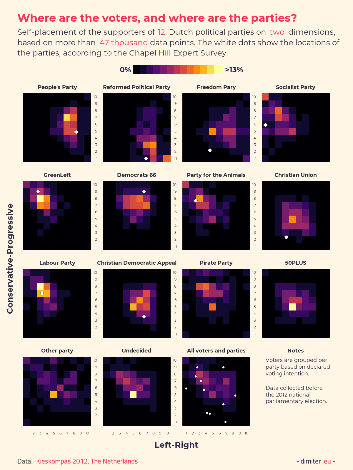
The figure shows that there is considerable variation in the self-placement for the supporters of all parties, but some in particular have very high spreads (e.g. the PVV). It is also noteworthy that people are reluctant to pick the extremes, especially when it comes to the Right and Conservative ends of the spectrum. Also, the party positions based on the Chapel Hill Expert Survey tend to be more extreme than the center of gravity of the positions of the voters of that party (not in all cases, though).
Objective policy positions I (induction)
The self-placements are interesting, but they only reveal the subjective positions of the voters. We do not know what the content of these positions is, and how they relate to actual positions on concrete policy issues. Fortunately, the VAA also contains data on the positions of the users on 30 policy issues. Positions are expressed in relation to statements, such as ‘The Netherlands should stay the Eurozone’ and ‘All coffeeshops should be closed’. Positions are recorded on a 5-point scale from ‘Strongly Disagree’ to ‘Strongly Agree’, with a ‘Neutral’ category.
So are these policy positions structured? If the Left/Right and Conservative/Progressive labels are meaningful, we would expect that a large part of the variation in responses can be summarized by two dimensions (factors) that contain policy items clearly related to these labels.
We can use a data reduction/structure detection technique, such as Principal Component Analysis, Factor Analysis, or Item-Response Models, to answer such questions, but before we do that, it is instructive to look at the correlation matrix directly.
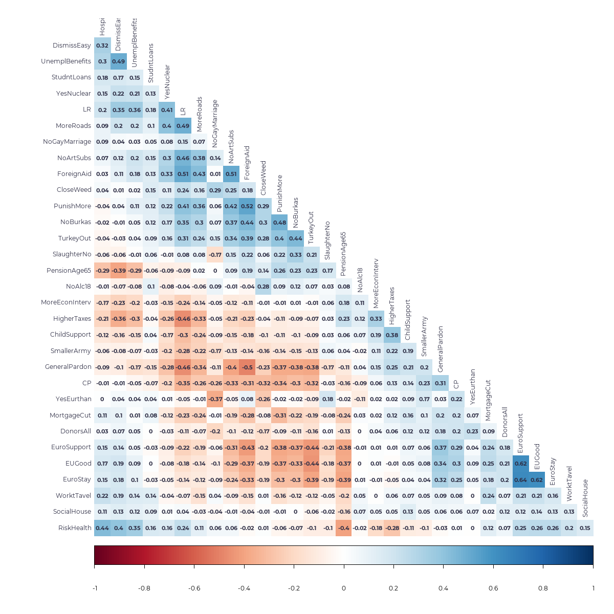
The correlation matrix reveals that there are altogether weak correlations and not many well-defined correlation clusters between the 30 items. There is one cluster related to questions about the EU and the euro (items EuroStay, EUGood, and EuroSupport) that has correlations in excess of 0.60. There is another cluster, including the items TurkeyOut, NoBurkas, PunishMore, ForeignAid(less), NoArtSubs(idies) and possibly GeneralPardon and MoreRoads, with correlations around 0.40. And there is a small cluster of economic-related items (UnemplBenefits(cut),DismissEasy, HospitalStay(payfor), possibly PensionAge) with correlations between 0.3 and 0.5. But, overall, the correlations between the items are weak and without clear patterns.
Let’s factor analysis explore these patterns further. The first decision is how many factors to retain, but this is not quite clear. Different criteria suggest anything between 2 and 6. Altogether, a four-factor solution seems to work best in terms of interpretability and maximizing the share of items that load highly on one factor at least. To enhance interpretability, we should allow for rotation of the factors. Promax oblique rotation of the factors is preferred to orthogonal rotations like varimax, as the factors should be allowed to be correlated (the two self-placement dimensions are correlated at -0.34.) Because of the limited scale of variation of the item response scales (5 levels), we better use a covariance matrix based on polychoric correlations. Below, I report a 4-factor solution with promax rotation and polichoric correlations, but variation in these options does not produce hugely different results.
tk1<-as.data.frame(tk)[, c(n3,n4, n2:(n2+1), n2a:(n2a+1),  n2b:(n2b+1), c(n:(n+29)))]
tk1<-tk1[complete.cases(tk1),]
fita4p <- fa.poly(tk1[,-c(1:8)], nfactors=4, scores="tenBerge", rotate='Promax')
print(fita4p, digits=2, cut=.3, sort=T)
## Factor Analysis using method = minres
## Call: fa.poly(x = tk1[, -c(1:8)], nfactors = 4, rotate = "Promax",
## scores = "tenBerge")
## Standardized loadings (pattern matrix) based upon correlation matrix
## item MR1 MR4 MR2 MR3 h2 u2 com
## ForeignAid 22 0.77 0.66 0.34 1.3
## PunishMore 7 0.75 0.54 0.46 1.0
## NoBurkas 24 0.72 0.50 0.50 1.0
## EuroSupport 3 -0.64 0.36 0.58 0.42 1.6
## TurkeyOut 4 0.61 0.45 0.55 1.1
## NoArtSubs 26 0.60 0.44 0.56 1.3
## EUGood 2 -0.57 0.41 0.57 0.43 1.9
## EuroStay 1 -0.57 0.41 0.55 0.45 2.0
## GeneralPardon 25 -0.56 0.47 0.53 1.5
## SlaughterNo 11 0.47 0.24 0.76 2.0
## MoreRoads 9 0.42 -0.42 0.41 0.59 2.2
## MortgageCut 20 -0.31 0.23 0.77 2.7
## RiskHealth 14 0.63 -0.30 0.48 0.52 1.6
## DismissEasy 18 0.59 -0.40 0.50 0.50 1.8
## HospitalStay 15 0.55 0.36 0.64 1.5
## PensionAge65 17 0.38 -0.52 0.33 0.52 0.48 2.6
## UnemplBenefits 19 0.51 -0.36 0.41 0.59 2.0
## WorktTavel 10 0.43 0.25 0.75 1.8
## StudntLoans 12 0.39 0.20 0.80 1.8
## SocialHouse 21 0.33 0.16 0.84 1.9
## HigherTaxes 16 0.70 0.54 0.46 1.2
## ChildSupport 13 0.52 0.32 0.68 1.2
## MoreEconInterv 29 0.43 0.20 0.80 1.2
## YesNuclear 27 -0.39 0.29 0.71 2.4
## NoAlc18 28 0.36 0.20 0.80 2.4
## SmallerArmy 23 0.19 0.81 2.2
## YesEurthan 30 0.69 0.46 0.54 1.1
## NoGayMarriage 6 -0.66 0.42 0.58 1.1
## CloseWeed 8 0.34 -0.53 0.48 0.52 2.2
## DonorsAll 5 0.37 0.21 0.79 1.6
##
## MR1 MR4 MR2 MR3
## SS loadings 4.91 2.82 2.42 1.70
## Proportion Var 0.16 0.09 0.08 0.06
## Cumulative Var 0.16 0.26 0.34 0.39
## Proportion Explained 0.41 0.24 0.20 0.14
## Cumulative Proportion 0.41 0.65 0.86 1.00
##
## With factor correlations of
## MR1 MR4 MR2 MR3
## MR1 1.00 -0.09 -0.19 -0.27
## MR4 -0.09 1.00 0.03 0.11
## MR2 -0.19 0.03 1.00 0.14
## MR3 -0.27 0.11 0.14 1.00
##
## Mean item complexity = 1.7
## Test of the hypothesis that 4 factors are sufficient.
##
## The degrees of freedom for the null model are 435 and the objective function was 10.2 with Chi Square of 438215
## The degrees of freedom for the model are 321 and the objective function was 1.17
##
## The root mean square of the residuals (RMSR) is 0.03
## The df corrected root mean square of the residuals is 0.04
##
## The harmonic number of observations is 42955 with the empirical chi square 39740.25 with prob < 0
## The total number of observations was 42955 with Likelihood Chi Square = 50403.67 with prob < 0
##
## Tucker Lewis Index of factoring reliability = 0.845
## RMSEA index = 0.06 and the 90 % confidence intervals are 0.06 0.061
## BIC = 46979.28
## Fit based upon off diagonal values = 0.98
## Measures of factor score adequacy
## MR1 MR4 MR2 MR3
## Correlation of (regression) scores with factors 0.95 0.89 0.88 0.87
## Multiple R square of scores with factors 0.90 0.79 0.77 0.75
## Minimum correlation of possible factor scores 0.81 0.59 0.53 0.50The total explained variance is 39%, with the four factors accounting for 16%, 9%, 8%, and 6% respectively. The correlation between the first and the fourth factor is rather high (note the confusing labeling of the factor names in the output of the analysis). The first factor is rather mixed and relates to nativist items (less foreign aid, no Turkey in the EU, no ritual slaughter of animals, ban on burkas, no general pardon for migrant kids), with anti-elite (no art subsidies), paternalistic (more severe punishments for small offences, closing down of coffeeshops), and other items, such as building more roads. Importantly, in a 5-factor solution, the EU and Euro-related items separate in their own factor.
The second factor relates to economic items: easier dismissal of workers, higher own-risk for health insurance, higher fees for hospital stays, increasing the pension age, reducing the unemployment benefits, and some others. We can term this factor economic liberalism. Importantly, not all economy-related items load highly on this dimension, and some of the EU ones load highly as well (but not uniquely).
The third factor relates to other economic items, including some of the ‘classic’ ones, such as support for more government intervention in the economy, higher taxes and lower child benefits for the rich. That’s why we can label it economic interventionism. But some of the highly-loading items don’t quite fit thematically this label, such as support for a ban on alcohol sales for youths under 18, and opposition to new nuclear stations.
The fourth item relates to moral permisiveness items, such as support for legal euthanasia and automatic donor registrations and opposition to civil servants being able to refuse to register same-sex marriages and closing down of coffee shops. Interestingly, the item related to ban on sale of alcohol does not load highly here, although one would expect it to be related.
Let’s explore in more detail how the factors correlate with the left/right and conservative/progressive self-placements below. On the basis of the factor loadings, we can already note that the first, most prominent, factor does not map directly on classic interpretations of left/right. It misses most economic items, as well as the classic progressive morality issues. It is also remarkable that the economic items split on two, uncorrelated dimensions, with the ‘classic’ items loading on the smaller one (in terms of explained variance). Looking at the figure below, we can see that left/right self-placements are moderate correlated with the first and the third factor, conservative-progressive self-placements are moderately correlated with the first and the fourth factor, and the second factor is not correlated strongly with either. So the first factor captures some but not all elements from the subjective dimensions, and the second factor is not captured well at all.

The analysis above is based on the close to 43,000 records that have complete data on all 30 policy items, plus the self-placements, and party voting intention. When we run the analysis on the more than 500,000 records that have completed only the policy items, the results are remarkably similar, with the factors being even crisper, even if the explained variance drops slightly.
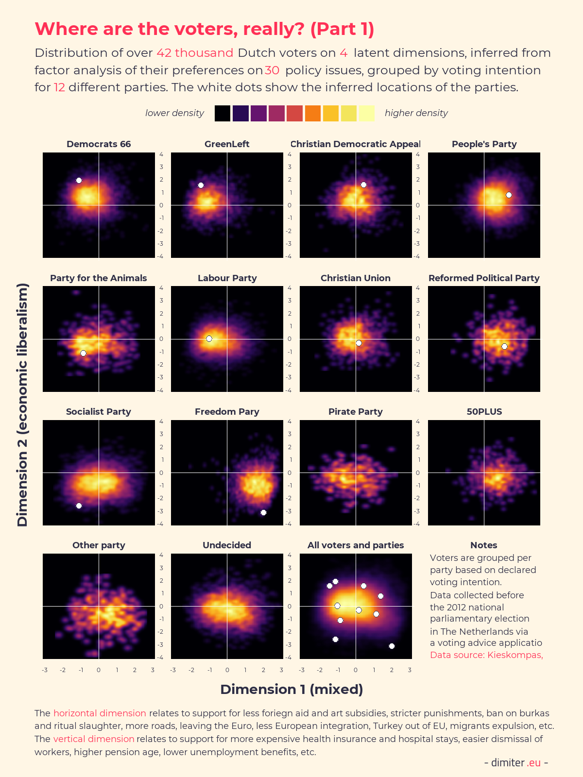
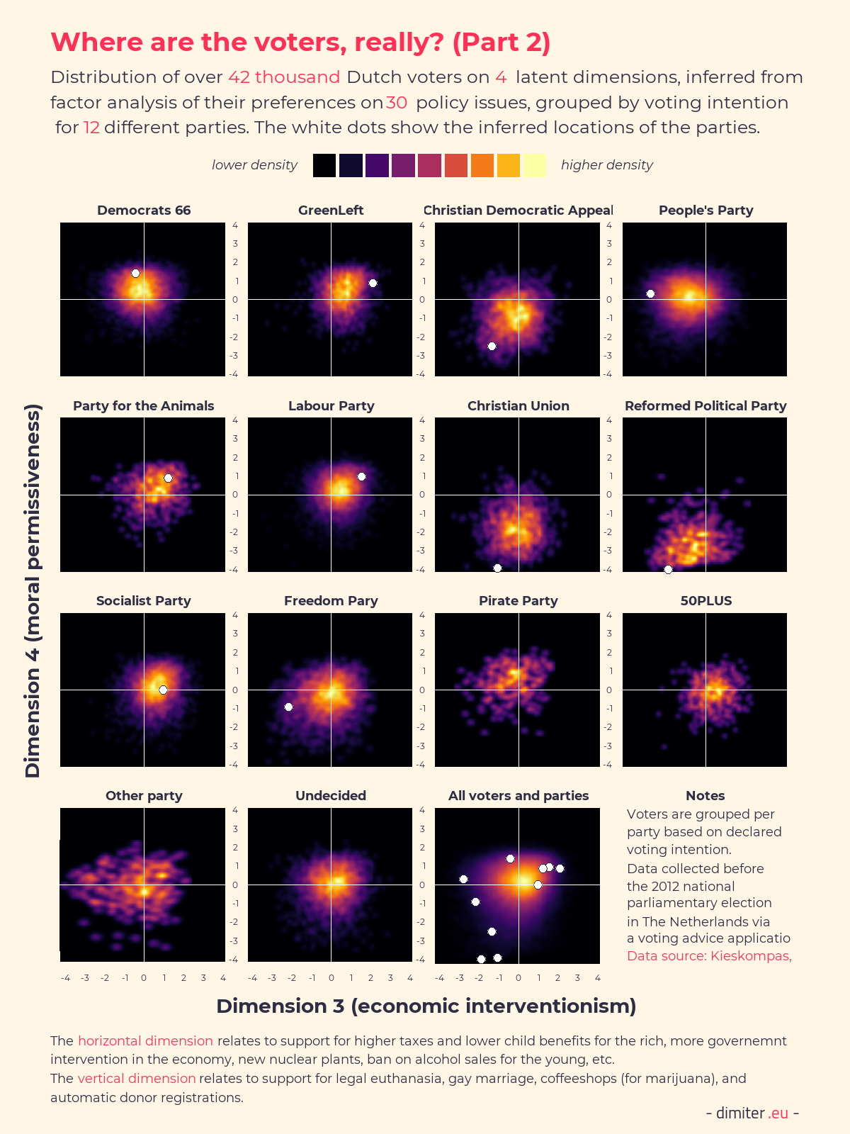
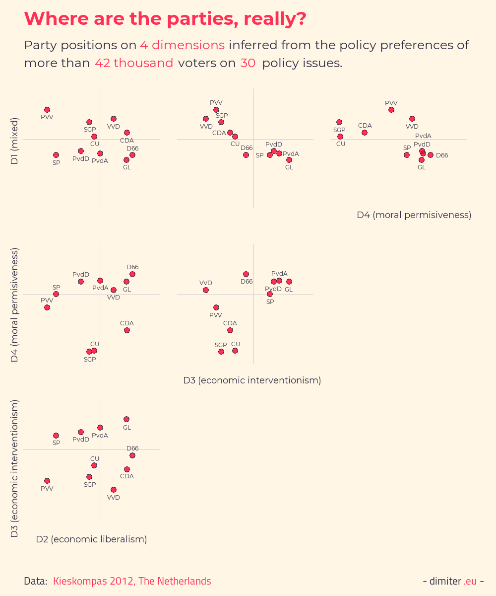
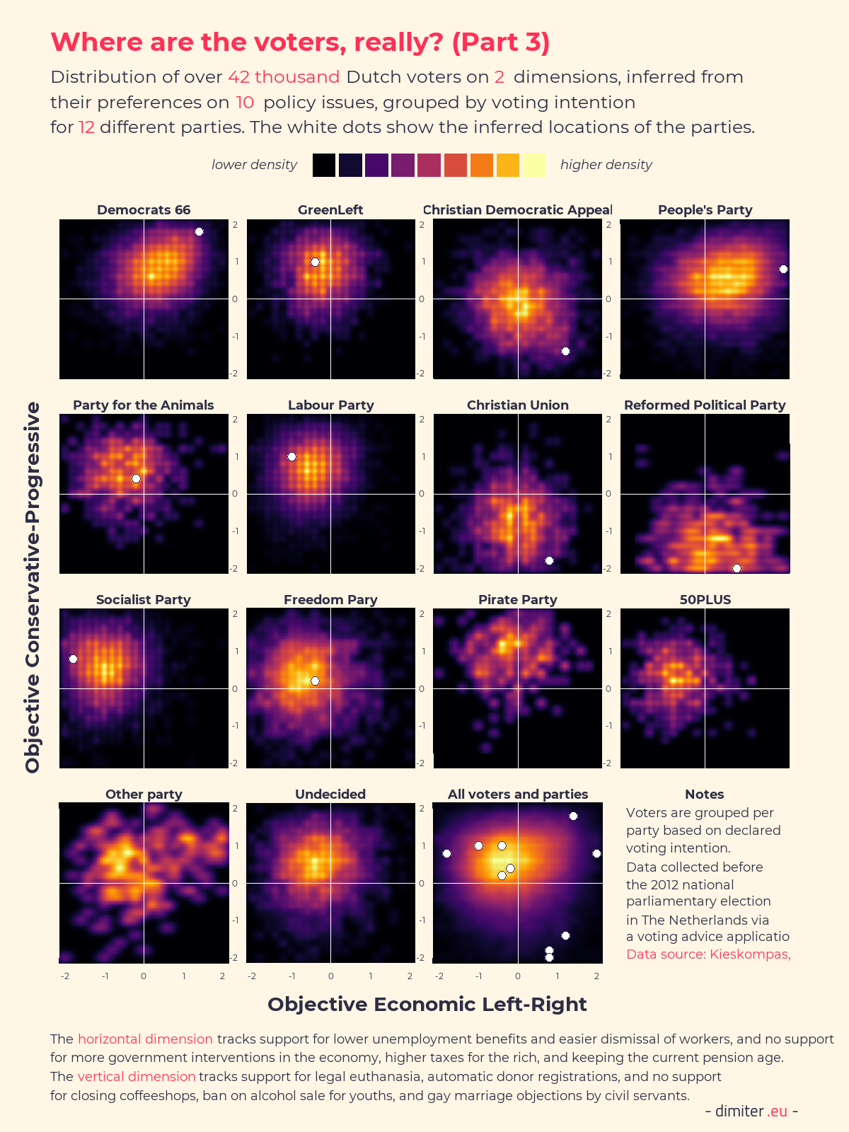
Having the identified the four factors, we can compute factor scores for each individual in the data on each of the four dimensions. Because we also have the party positions on the 30 policy items, we can also assign the parties scores on these same dimensions, so that we can compare the voters and the parties in the same space. The following two figures show heatmaps of the distributions, with the positions of the parties indicated by the white dots. (Data on the positions of the 50+ and the Pirates party is not available, unfortunately.)
What we can see is that the voters of different parties are much more separated based on their policy positions, as summarized by their factor scores, then by the self-placements. For example, the Freedom party voters are almost all in the bottom-right corner on the first two dimensions and the GreenLeft voters are almost all in the top-right corner on the second pair of dimensions. It is instructive to compare the spread of the voters as well, with some groups being quite compact (on some of the dimensions) and rather spread-out on others. It is quite remarkable that in almost all cases the party positions are more extreme than the positions of their voters, and in some cases greatly so.
The next figure focuses on the placement of the parties only, and shows the positions for each pair of the four dimensions to highlight the correlations and lack thereof. Only on plot showing economic interventionism vs. the mixed first factor, the party positions line-up on an almost straight line. This suggests that the party political space might be simpler than the voters’ one, but comparisons are difficult due to the very different number of cases in the subsets of parties and voters.
‘Objective’ positions based on policy preferences: deductive approach
We can have concerns about whether the inferred dimensions are really what should define the voters’ positions. After all, we can ask why these 30 items and not some others, or to reasons that some of these policies are more important than others. So we can do something different than the inductive factor-analytic approach: we can define ‘deductively’ which items define the left/right and conservative/progressive dimensions, and simply average the answers of the voters and the parties on these ‘deductively-defined’ dimensions. For left/right, the five items that I choose as most important and directly related are support for lower unemployment benefits and easier dismissal of workers, and no support for more government interventions in the economy, higher taxes for the rich, and keeping the current pension age. For the conservative/progressive dimension I choose support for legal euthanasia, automatic donor registrations, and no support for closing coffeeshops, ban on alcohol sale for youths, and gay marriage objections by civil servants. Note that this is my interpretation of what is most important and at the heart of these dimensions, and other operationalizations are possible. The figure below shows the distribution of voters and parties on these two ‘deductively’ defined policy preference dimensions.
The picture we see is rather similar to the ones with the inductively inferred factor-analytic dimensions. The match with the self-placement is rather poor. The correlation between the self-placement on left/right and the ‘objective’ left/right scores is 0.45. For the conservative-progressive dimensions, the correlation is 0.36. Not negligible, but far from deterministic.
Conclusion
What did we learn? The major take-aways from the analysis are that:
Subjective self-placements are not directly and strongly related to actual preferences over policies. They are rather variable within groups of party supporters and tend to gravitate towards the center.
Voters positions inferred from their expressed preferences over policies are complexly structured in a way that we need at least four dimensions to capture the main dimensions of variation, which still leaves a lot of variation unaccounted for. The structure is not what one would expect under the assumption of a classic two-dimensional space, not only in terms of number of dimensions, but also in their content. These dimensions separate groups of party supporters better.
Parties are almost always more extreme than their voters, to some extent when it comes to self/expert-placements, but remarkably so when we look at their actual positions, either by inductively identifying dimensions or by deductively defining what goes into the left/right and conservative/progressive dimensions. When we position the parties in the space defined by the voters’ preferences, some suspected but unconfirmed similarities and differences between the parties emerge, such as the proximity between the Freedom Party and the Socialist Party on the economic liberalism dimension.
Finally, a reminder that all this is based on a non-probability sample of one country for one particular time period, so we should be careful with generalizations beyond this context.